10X Example

Last updated: 2018-09-14

workflowr checks: (Click a bullet for more information)

✔ R Markdown file: up-to-date

Great! Since the R Markdown file has been committed to the Git repository, you know the exact version of the code that produced these results.
✔ Environment: empty

Great job! The global environment was empty. Objects defined in the global environment can affect the analysis in your R Markdown file in unknown ways. For reproduciblity it’s best to always run the code in an empty environment.
✔ Seed: set.seed(20180618)

The command set.seed(20180618) was run prior to running the code in the R Markdown file. Setting a seed ensures that any results that rely on randomness, e.g. subsampling or permutations, are reproducible.
✔ Session information: recorded

Great job! Recording the operating system, R version, and package versions is critical for reproducibility.

✔ Repository version: 86bd1c0

Great! You are using Git for version control. Tracking code development and connecting the code version to the results is critical for reproducibility. The version displayed above was the version of the Git repository at the time these results were generated.

Note that you need to be careful to ensure that all relevant files for the analysis have been committed to Git prior to generating the results (you can use wflow_publish or wflow_git_commit). workflowr only checks the R Markdown file, but you know if there are other scripts or data files that it depends on. Below is the status of the Git repository when the results were generated:


Ignored files:
    Ignored:    .Rhistory
    Ignored:    .Rproj.user/
    Ignored:    R/.Rhistory
    Ignored:    analysis/.Rhistory
    Ignored:    analysis/pipeline/.Rhistory

Untracked files:
    Untracked:  ..gif
    Untracked:  .DS_Store
    Untracked:  R/.DS_Store
    Untracked:  analysis/.DS_Store
    Untracked:  analysis/normalization_test.R
    Untracked:  analysis/pipeline/0_dropseq/
    Untracked:  analysis/pipeline/1_10X/
    Untracked:  analysis/pipeline/2_zeisel/
    Untracked:  analysis/pipeline/3_smallsets/
    Untracked:  analysis/slsl_10x.Rdata
    Untracked:  analysis/slsl_dropseq.Rdata
    Untracked:  analysis/writeup/bibliography.bib
    Untracked:  analysis/writeup/draft1.aux
    Untracked:  analysis/writeup/draft1.bbl
    Untracked:  analysis/writeup/draft1.blg
    Untracked:  analysis/writeup/draft1.log
    Untracked:  analysis/writeup/draft1.out
    Untracked:  analysis/writeup/draft1.pdf
    Untracked:  analysis/writeup/draft1.synctex.gz
    Untracked:  analysis/writeup/draft1.tex
    Untracked:  analysis/writeup/jabbrv-ltwa-all.ldf
    Untracked:  analysis/writeup/jabbrv-ltwa-en.ldf
    Untracked:  analysis/writeup/jabbrv.sty
    Untracked:  analysis/writeup/naturemag-doi.bst
    Untracked:  analysis/writeup/wlscirep.cls
    Untracked:  data/unnecessary_in_building/
    Untracked:  docs/figure/10x_labeled.Rmd/
    Untracked:  docs/figure/example_10x.Rmd/.DS_Store
    Untracked:  docs/figure/small.Rmd/
    Untracked:  dropseq_heatmap.pdf
    Untracked:  man/correct_detection_rate.Rd

Unstaged changes:
    Modified:   NAMESPACE
    Modified:   R/SLSL.R
    Modified:   R/correct_detection_rate.R
    Modified:   R/find_markers.R
    Modified:   analysis/pipeline/.DS_Store
    Modified:   analysis/writeup/.DS_Store
    Modified:   data/.DS_Store
    Modified:   docs/figure/.DS_Store
    Deleted:    man/correct.detection.rate.Rd

Note that any generated files, e.g. HTML, png, CSS, etc., are not included in this status report because it is ok for generated content to have uncommitted changes.

Expand here to see past versions:

File	Version	Author	Date	Message
Rmd	86bd1c0	tk382	2018-09-14	wflow_publish(c(“analysis/_site.yml“,”analysis/large.Rmd“,”analysis/small.Rmd“), republish
html	32ed2c0	tk382	2018-09-13	small edits
Rmd	047143d	tk382	2018-09-12	large set pipeline
html	047143d	tk382	2018-09-12	large set pipeline
Rmd	03a7f75	tk382	2018-09-12	notation change, adding visualization, general code structure

Load Package

Read Data : PBMC 27K

Read data and keep the gene names separately.

orig = readMM('data/unnecessary_in_building/pbmc3k/matrix.mtx')
orig_genenames = read.table('data/unnecessary_in_building/pbmc3k/genes.tsv',
                            stringsAsFactors = FALSE)$V2

Quality Control and Cell Filtering

First, “explore.data” function shows the distribution of the number of UNI, detection rate, and the proportion of mitochondrial genes for each cell. Then users can decide on the cut-offs to filter the cells using “cell.filter” function, which returns the indices of cells that satisfy the input criteria.

summary = explore_data(orig, orig_genenames)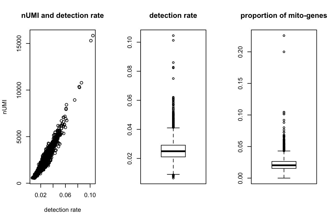

ind = cell_filter(summary, 
                  nUMI.thresh = c(0,10000), 
                  det.rate.thresh = c(0.02, 0.067), 
                  percent.mito.thresh = c(0,0.1))
tmpX = orig[,ind]

Gene Filtering

Next find variable genes using normalized dispersion. First, “plot.dispersion” function shows the distribution log of normalized dispersion (variance to mean ratio) against the gene means. The convention is to normalize the dispersion by converting them to z-scores, but one can also use median and MAD (median absolute deviation) which is less sensitive to outliers. Based on the scatterplot, users can decide on the cut-offs for the mean expression value and the dispersion to use “gene.filter” function. “gene.filter” function returns the new expression level matrix of filtered genes and the corresponding gene names.

disp = plot_dispersion(X = tmpX, 
                       genenames = orig_genenames, 
                       bins=NA, 
                       median = FALSE, 
                       outliers.mean.thresh = c(30,Inf),
                       outliers.vmr.thresh = c(3,Inf))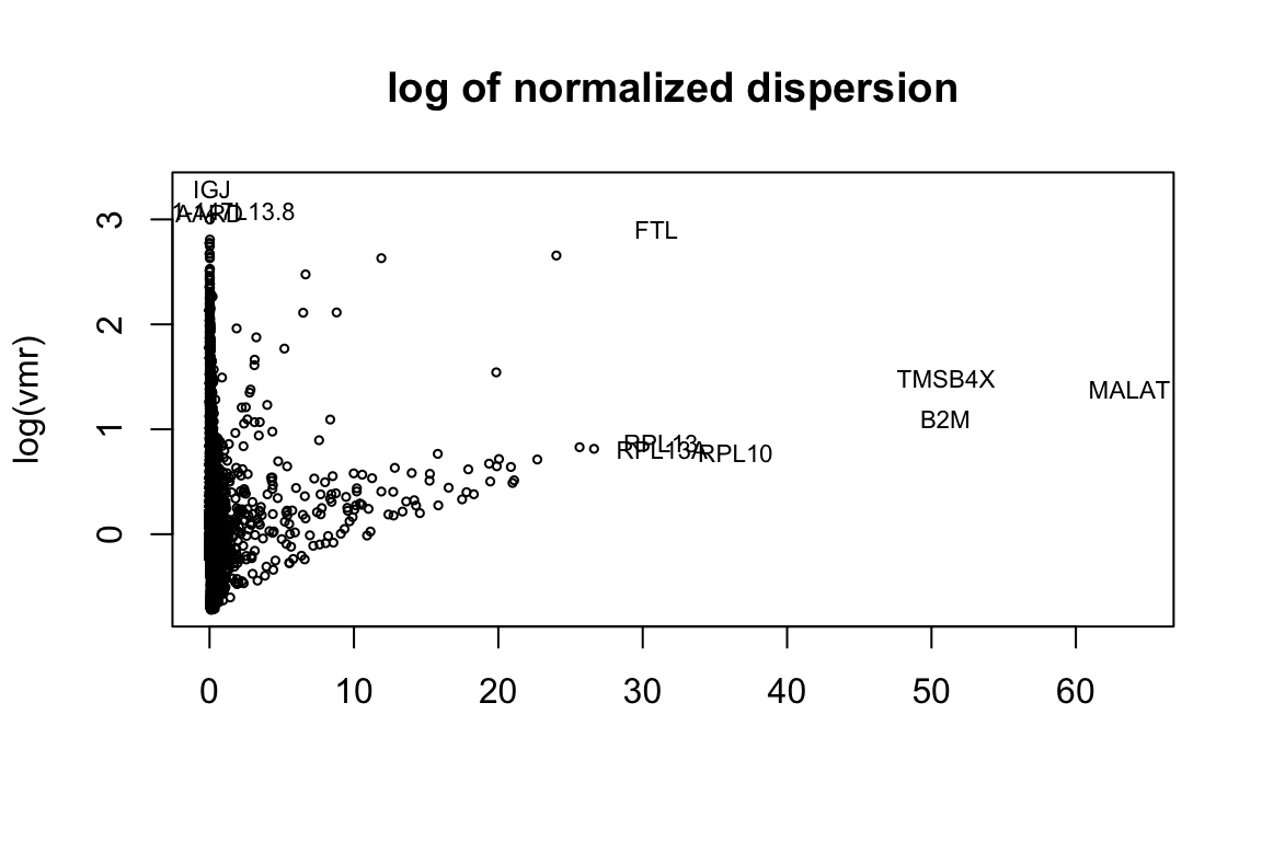

X = gene_filter(tmpX, orig_genenames, disp, 
                mean.thresh=c(0.001, Inf), 
                dispersion.thresh = c(0.5, Inf))
genenames = X$genenames
X = X$X

UMI Normalization

Use quantile-normalization to make the distribution of each cell the same. “quantile.normalize” function also performs the log transformation.

X = quantile_normalize(as.matrix(X))

Run SLSL

Run the clustering algorithm SLSL based on the filtered matrix. It automatically plots the final tSNE plot based on the Laplacian matrix.

out = SLSL(X, verbose=FALSE)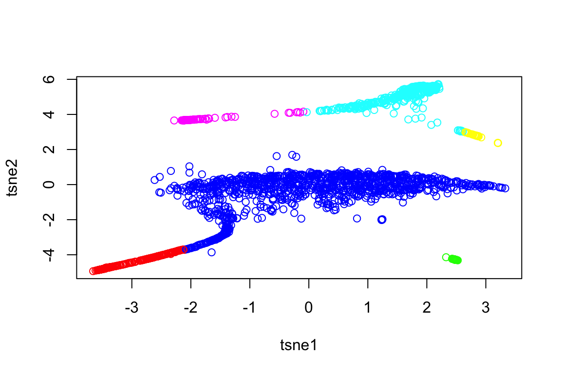

Differentially Expressed Genes

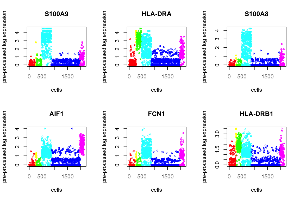
Using Kruskal test, we order the p-values to find the top differentially expressed genes. Below we present 6.

degenes = de_genes(X, genenames, out$result, top.n=100, plot=12)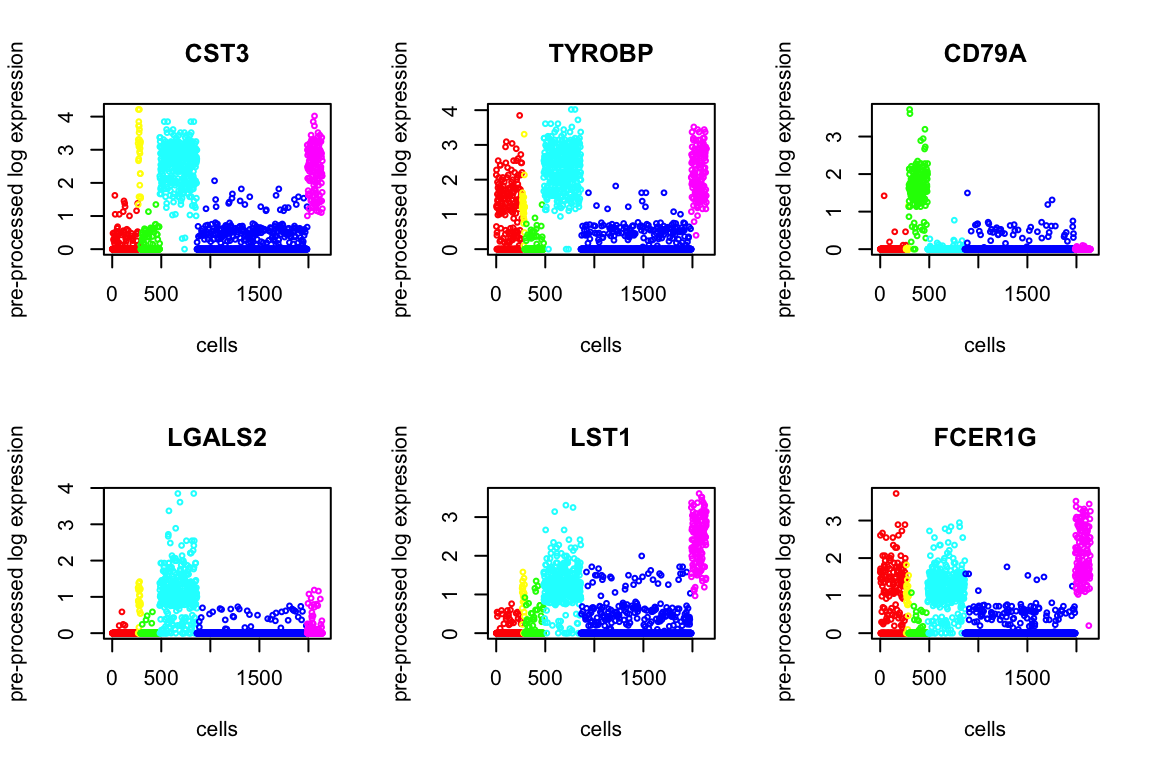

head(degenes)

  de_genes   log10p
1     CST3      Inf
2   TYROBP      Inf
3    CD79A      Inf
4   LGALS2      Inf
5     LST1 322.2270
6   FCER1G 314.1417

Markers for Each Cluster

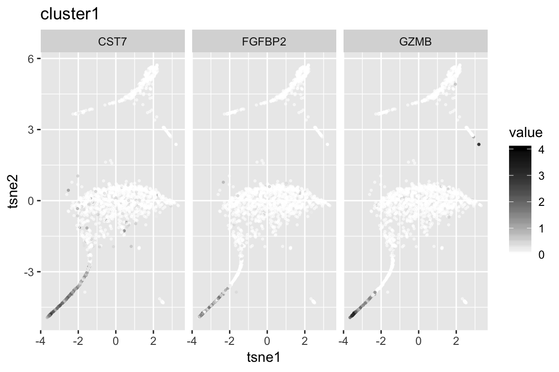
  clust1_genenames clust1_log10p
1             GZMB      280.5690
2           FGFBP2      249.4204
3             CST7      239.9105
4             PRF1      220.0278
5             NKG7      213.0282
6             CCL4      167.3846

  clust2_genenames clust2_log10p
1         SERPINF1     152.41836
2           FCER1A     143.19380
3             ENHO      79.10624
4           CLEC4C      77.80362
5           LRRC26      52.64777
6              SCT      52.64777

  clust3_genenames clust3_log10p
1            CD79A           Inf
2         HLA-DQA1      181.1766
3            CD79B      178.5284
4         HLA-DQB1      147.7264
5            FCRLA      134.5673
6             CD74      105.0767

  clust4_genenames clust4_log10p
1           LGALS2           Inf
2           S100A8      297.9284
3           S100A9      259.9251
4             FCN1      250.8238
5              LYZ      207.8968
6             CST3      204.0437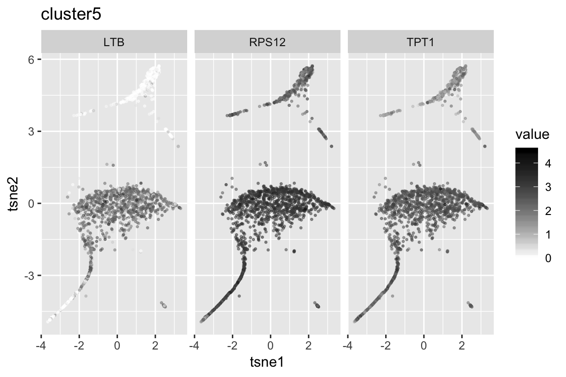

  clust5_genenames clust5_log10p
1             TPT1      203.0014
2              LTB      202.5040
3            RPS12      192.9751
4           RPS27A      165.8921
5           RPL10A      164.1815
6             RPS5      154.5735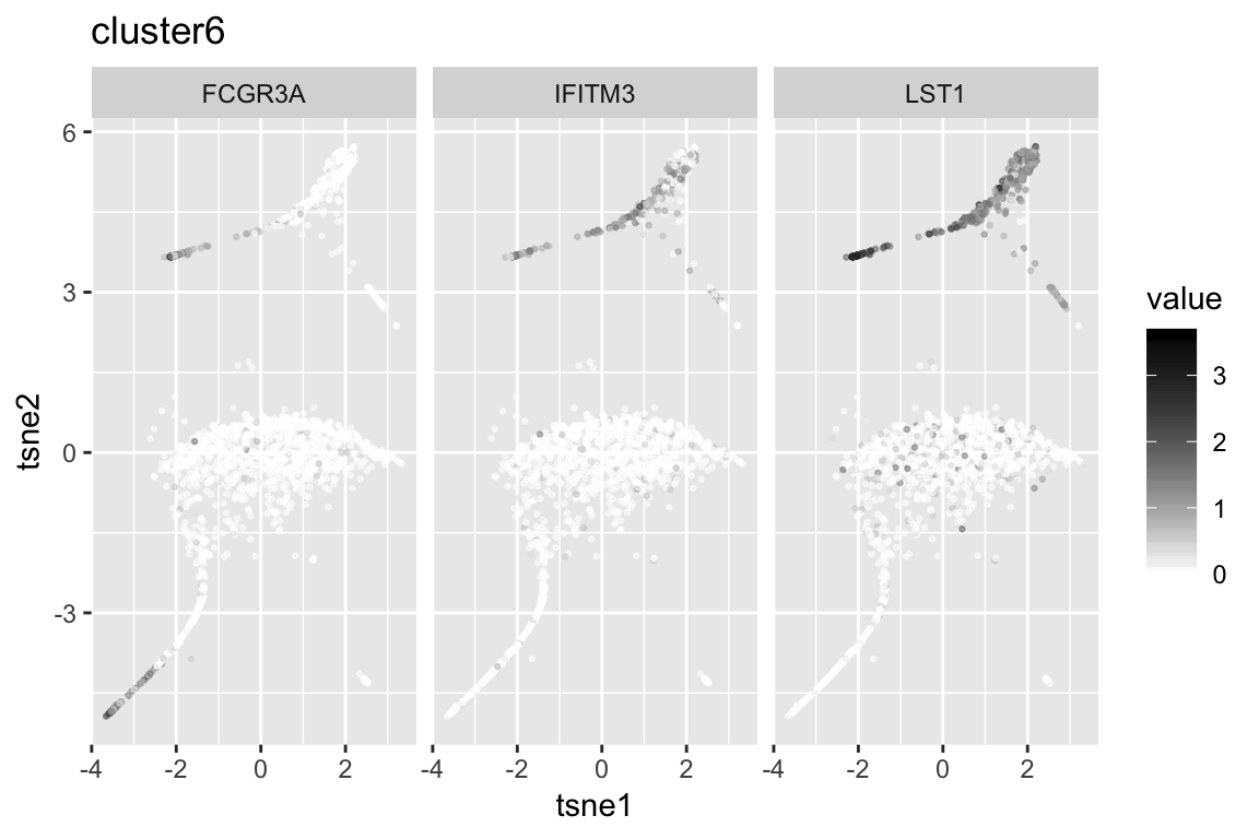

  clust6_genenames clust6_log10p
1           FCGR3A     144.34980
2           IFITM3     124.06185
3             LST1     118.87115
4             AIF1     107.61418
5           FCER1G     107.49510
6            C5AR1      77.95185

Session information

sessionInfo()

R version 3.5.1 (2018-07-02)
Platform: x86_64-apple-darwin15.6.0 (64-bit)
Running under: macOS Sierra 10.12.5

Matrix products: default
BLAS: /Library/Frameworks/R.framework/Versions/3.5/Resources/lib/libRblas.0.dylib
LAPACK: /Library/Frameworks/R.framework/Versions/3.5/Resources/lib/libRlapack.dylib

locale:
[1] en_US.UTF-8/en_US.UTF-8/en_US.UTF-8/C/en_US.UTF-8/en_US.UTF-8

attached base packages:
[1] parallel  stats4    stats     graphics  grDevices utils     datasets 
[8] methods   base     

other attached packages:
 [1] bindrcpp_0.2.2              gridExtra_2.3              
 [3] SC3_1.8.0                   SingleCellExperiment_1.2.0 
 [5] SummarizedExperiment_1.10.1 DelayedArray_0.6.2         
 [7] BiocParallel_1.14.2         Biobase_2.40.0             
 [9] GenomicRanges_1.32.6        GenomeInfoDb_1.16.0        
[11] IRanges_2.14.10             S4Vectors_0.18.3           
[13] BiocGenerics_0.26.0         SCNoisyClustering_0.1.0    
[15] plotly_4.8.0                gplots_3.0.1               
[17] diceR_0.5.1                 Rtsne_0.13                 
[19] igraph_1.2.2                scatterplot3d_0.3-41       
[21] pracma_2.1.4                fossil_0.3.7               
[23] shapefiles_0.7              foreign_0.8-71             
[25] maps_3.3.0                  sp_1.3-1                   
[27] caret_6.0-80                lattice_0.20-35            
[29] reshape_0.8.7               dplyr_0.7.6                
[31] quadprog_1.5-5              inline_0.3.15              
[33] matrixStats_0.54.0          irlba_2.3.2                
[35] Matrix_1.2-14               plyr_1.8.4                 
[37] ggplot2_3.0.0               MultiAssayExperiment_1.6.0 

loaded via a namespace (and not attached):
  [1] backports_1.1.2           workflowr_1.1.1          
  [3] lazyeval_0.2.1            splines_3.5.1            
  [5] digest_0.6.15             foreach_1.4.4            
  [7] htmltools_0.3.6           gdata_2.18.0             
  [9] magrittr_1.5              cluster_2.0.7-1          
 [11] doParallel_1.0.11         ROCR_1.0-7               
 [13] sfsmisc_1.1-2             recipes_0.1.3            
 [15] gower_0.1.2               dimRed_0.1.0             
 [17] R.utils_2.6.0             colorspace_1.3-2         
 [19] rrcov_1.4-4               WriteXLS_4.0.0           
 [21] crayon_1.3.4              RCurl_1.95-4.11          
 [23] jsonlite_1.5              RcppArmadillo_0.8.600.0.0
 [25] bindr_0.1.1               survival_2.42-6          
 [27] iterators_1.0.10          glue_1.3.0               
 [29] DRR_0.0.3                 registry_0.5             
 [31] gtable_0.2.0              ipred_0.9-6              
 [33] zlibbioc_1.26.0           XVector_0.20.0           
 [35] kernlab_0.9-26            ddalpha_1.3.4            
 [37] DEoptimR_1.0-8            abind_1.4-5              
 [39] scales_0.5.0              mvtnorm_1.0-8            
 [41] pheatmap_1.0.10           rngtools_1.3.1           
 [43] bibtex_0.4.2              Rcpp_0.12.18             
 [45] viridisLite_0.3.0         xtable_1.8-2             
 [47] magic_1.5-8               mclust_5.4.1             
 [49] lava_1.6.2                prodlim_2018.04.18       
 [51] htmlwidgets_1.2           httr_1.3.1               
 [53] RColorBrewer_1.1-2        pkgconfig_2.0.1          
 [55] R.methodsS3_1.7.1         nnet_7.3-12              
 [57] labeling_0.3              later_0.7.3              
 [59] tidyselect_0.2.4          rlang_0.2.1              
 [61] reshape2_1.4.3            munsell_0.5.0            
 [63] tools_3.5.1               pls_2.6-0                
 [65] broom_0.5.0               evaluate_0.11            
 [67] geometry_0.3-6            stringr_1.3.1            
 [69] yaml_2.2.0                ModelMetrics_1.1.0       
 [71] knitr_1.20                robustbase_0.93-2        
 [73] caTools_1.17.1.1          purrr_0.2.5              
 [75] nlme_3.1-137              doRNG_1.7.1              
 [77] mime_0.5                  whisker_0.3-2            
 [79] R.oo_1.22.0               RcppRoll_0.3.0           
 [81] compiler_3.5.1            e1071_1.7-0              
 [83] tibble_1.4.2              pcaPP_1.9-73             
 [85] stringi_1.2.4             pillar_1.3.0             
 [87] data.table_1.11.4         bitops_1.0-6             
 [89] httpuv_1.4.5              R6_2.2.2                 
 [91] promises_1.0.1            KernSmooth_2.23-15       
 [93] codetools_0.2-15          MASS_7.3-50              
 [95] gtools_3.8.1              assertthat_0.2.0         
 [97] CVST_0.2-2                pkgmaker_0.27            
 [99] rprojroot_1.3-2           withr_2.1.2              
[101] GenomeInfoDbData_1.1.0    grid_3.5.1               
[103] rpart_4.1-13              timeDate_3043.102        
[105] tidyr_0.8.1               class_7.3-14             
[107] rmarkdown_1.10            git2r_0.23.0             
[109] shiny_1.1.0               lubridate_1.7.4

This reproducible R Markdown analysis was created with workflowr 1.1.1